Simulation

Simulation

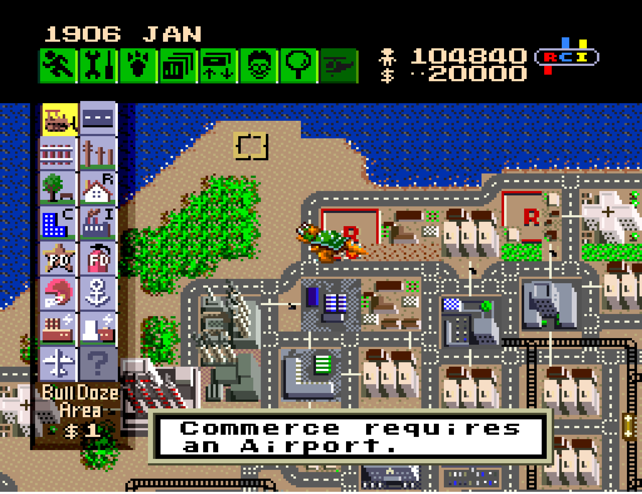
Computer simulations are useful. Scientists use them for climate modeling and protien folding. Engineers simulate materials, and bridges, and areodynamics. Video games simulate physics, enemy behaviors, or even entire cities. Simulations are used to model the stock market, assess risks, and optimize supply chains, and predict epidemics.

More importantly, computer simulations are fun. Video games are largely simulation and coding small, personal videogames is one of the most fun things you can do on a computer. I particularly value coding simulations to explore ideas. What better way is there to gain an understanding of how something works than to make it work yourself.

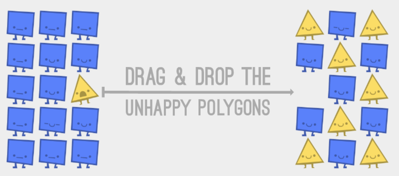
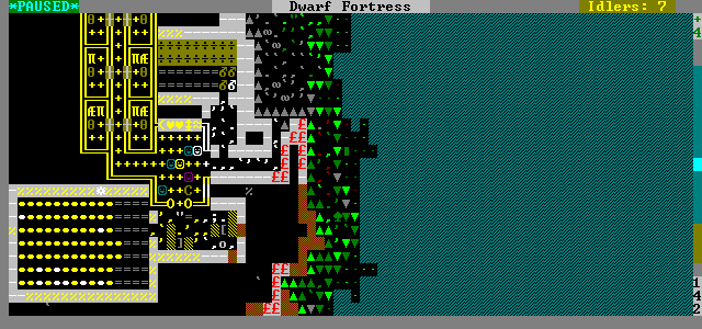
Computer simulation is a broad term, and lots of things with different structures fall into it. In this chapter we explore a three different types: physics simulation, cellular automata, artifical life. As different as these are, they all share a common core idea: represent a system with data, and iteratively update the system by applying rules.

Will Wright

SimCity, Maxis, 1989

One of the most well known simulation games, SimCity allows players to build and manage a city without a predefined goal.

Vi Hart and Nicky Case

Parable of the Polygons

An _explorable_ essay that uses interactive simulations to explore how small biases can lead to large scale segregation.

Parable of the PolygonsProject Website

Dwarf Fortress

Tarn and Zach Adams

A deeply complex simulation game challenging players to manage a group of dwarves in a procedurally generated world.

Dwarf FortressOffical Website

Liam

Matter.js

Matter.js is a 2D physics engine for the web.

Matter.jsOfficial Website

John Conway

The Game of Life

A cellular automaton originally presented as recreational mathematics that has had long lasting impacts across various fields.

Mathematical GamesScientific American 1970

Physics

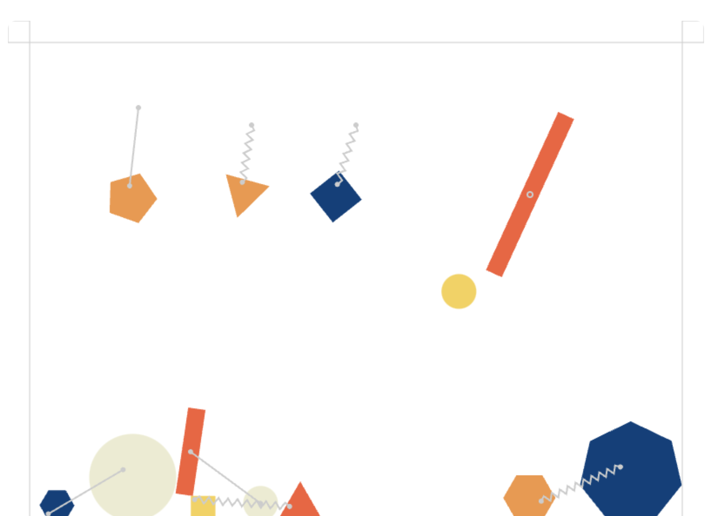
Perhaps the most commonly simulated system in video games is physics: how things move and collide. Some games, like racing sims, use principled, realistic physics. Some games, like Mario Brothers, use stylized phyiscs.

If you want to use physics in your own sketches, designs, games, and simulations you can use an existing physics library. There are lots of stand-alone 2D and 3D physics engines for most popular languages, and game engines like Unity and Godot usually include their own physics engine.

If you are making a medium- or large-scoped game, its probably a good idea to learn and use an full-featured, battle-tested physics engine. But for some projects and effects, you can code your own physics with just a few lines of code.

Position, Velocity, Acceleration

Three very important things in a physics simulation are position, velocity and acceleration.

Position Where it is. Velocity Direction and rate of change in position. Acceleration Direction and rate of change in velocity.

rate * time = distance

A blue bus travels down the road at 30 miles per hour. At 1 hour, it has traveled 30 miles. At 2 hours, it has traveled 60 miles.

acceleration * time = velocity

A red bus falls from a great height. The velocity increases linearly over time due to the const acceleration of gravity (9.8m/s^2). After 1 second the bus is moving at 9.8m/s. After 2 seconds the bus is moving 19.6m/s.

But how far does the red bus fall in 1 second? 2 seconds?

Analytical Integration

To find that out, we can use integration. Integration finds an accumulated value when we know how it changes over time. For example, we can find distance by integrating velocity and we can find velocity by integrating acceleration. Calculus provides the tools to analytically integrate. We can use it to derive equations for falling bodies. The folowing formula tells us how far an object falls for a given gravity and time.

.5 * gravity * time^2 = distance

At 1 second the bus has fallen 4.9 meters. At 2 seconds the bus has fallen 19.6 meters.

We’re gonna skip over how to use calculus to analytically integrate because 1) calculus is out of the scope of this chapter and 2) our simulations aren’t going to analytically integrate things anyway!

Numerical Integration

Above, we use a formula that tells us the distance an object will fall in a given amount of time. This formula was derived using calculus and analytical integration. It gives us an exact answer.

There is another approach we can use to estimate the answer instead: numerical integration. To perform numerical integration we break up time into small intervals, plug in the numbers for each interval, and calculate each change bit by bit.

Let’s use numerical integration to determine how far our bus falls in 2 seconds, using two 1 second intervals:

// starting values
acceleration = 9.8;
velocity = 0;
distance = 0;

// step forward 1 second
velocity += acceleration;
distance += velocity; // 9.8

// step forward 1 more second
velocity += acceleration; // 19.6
distance += velocity; // 29.4

Our estimate ends up being 29.4 meters, which is pretty far off from the exact value of 19.6 meters. It is pretty far off because it assumes that velocity is constant over each interval but actually the velocity continuously increases. With larger time intervals this error will be larger and the error accumulates over each step. 1 second intervals are too big.

Let’s try with .01 second intervals:

// starting values
acceleration = 9.8;
velocity = 0;
distance = 0;

for (let i = 0; i < 200; i++) {
  velocity += acceleration * 0.01;
  distance += velocity * 0.01;
}

console.log(distance); // 19.7

With .01 second intervals our estimate is 19.7, which is very close!

The numerical integration above uses the first-order Euler Method. This is a simple, but not very accurate, way to do numerical integration. You can increase accuracy by using more complex methods, but you don’t necessarily need to. Since the error is proportional to the step size, even the simple method above works well for small step sizes. Its “good enough” for a lot of simple simulations.

Simulation and Numerical Integration

Numerical integration is not as accurate as analytic integration in a simulation with multiple forces finding an analytic solution quickly becomes impossible. Numerical integration can handle this complexity and even account for real-time user input naturally. Let’s try it out with a few simple sims!

A Bouncing Ball

This example shows a pretty minimal bouncing ball. It simulates the effect of gravity on the velocity and position of the ball in one dimension. It also bounces the ball off the bottom of the canvas.

Some Bouncing Balls

This example increases the complexity of the simulation. It simulates multiple balls in two dimesions. It simulates gravity, air resistance, and inelastic collisions with the left, right, and bottom of the canvas. It doesn’t simulate collisions between balls.

Particles

This example shows an emitter/particle system. The simulation of the particles is very similar to the simulation of the balls in the example above.

Side note: This example uses a fixed pool of particles, recycling “dead” particles when creating new ones. This is a common optimization pattern in games to avoid creating short lived objects and reduce garbage collection performance issues.

A Chain

This example simulates gravity and spring forces on a chain of beads.

Simulation Error

This example simulates the path of a ball using numerical integration and analytic integration visualizing the estimation error.

Cellular Automata

Cellular automata are mathematical models comprising a grid of cells and a set of simple rules. In a cellular automata, cells are set to one of a finite set of states (e.g. on or off). A set of rules is then iteratively applied to every cell changing it’s state based on its current state and the states of its neighbors. They can be used to model things like crystal growth, fire spreading, and fluid dynamics.

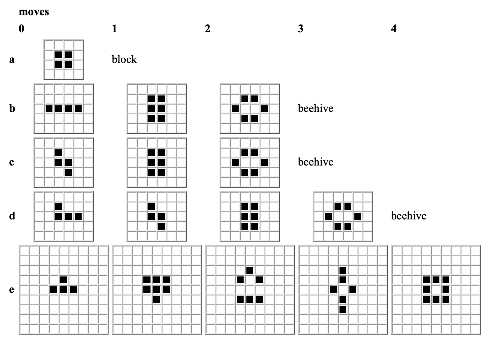
Cellular automata were invented in the 1940’s by Stanislaw Ulam (Monte Carlo Method, Manhattan Project) and John von Neumann (Game Theory, modern computer artchitecture, Manhattan Project). Conway’s Game of Life (1970) is likely the most famous cellular automata model. It is a simple system with just 2 states and 4 rules from which emerge rich and complex systems. The Game of Life is even Turing Complete meaning it can can follow instructions and compute.

Representing State in Images

The following examples keep track of the CA state as color values in a p5 graphics object’s pixel array. Representing CA state as an image is a pretty common technique, with some pros and cons.

The main disadvantage is that images are designed to store pixel color values not cell states. For a lot of cellular automata the state is a simple bit: on or off. Using a 24-bit RGB value to represent a single bit isn’t efficient. Depending on the kind of data you need to represent your states using an image might be awkward or simply not work.

The main advantage is that most programming environments have support for working with images built in. If you represent your state as an image it is easy to display: its an image, just draw it.

Most of the time, using an image works fine and sometimes you get some nice performance benefits since working with images is often optomized.

Cellular Automata Starter

This first example is models a simple growth. Cells can be in one of two states: off (represented by red value 0) and on (represented by red value > 0). The green and blue c_hannel values are not considered.

It starts out by creating a graphics object to hold the current state (g1) and draws a few white squares in it. It also creates a graphics object to hold the result of applying the rules (g2). You generally need to have two buffers like this so that you aren’t changing the values while you are reading them.

Cellular Automata Messy Growth

This example builds on Starter. It adds some randomness (cells don’t always turn on). It changes the on/off test to see if the pixel is black (off) or not (on). It sets the activated pixels to rainbow colors (any non=black color is “on”).

Cellular Color Copy

This example uses the same structure as the others. It starts by setting each pixel to a random color, then it follows a simple rule. Set each pixel to the color of one of its 4 neighbors, chosen at random.

Click the canvas to pause the simulation. I really like the images this once creates and the simplicity of the rule. I found this one by just playing around. Its similar to the Color War tweet-cart by Munro Hoberman.

Lines

This one looks for vertical and horizontal lines and extends them.

Game of Life

And finally, an implementation of Conway’s Game of Life. This example uses the same basic structure of all the others and implements the 4 simple Game of Life rules.

Microworlds

Mitchel Resnick (Creative Learning Spiral) published Turtles, Termites, and Traffic Jams in 1994. It discusses using computer “simulations” to explore ideas; introduces StarLogo a language he developed for this purpose; and provides several example simulations. He makes the point that “simulation” might not be the right word for these programs because the intent isn’t to model, imitate, and predict real-world systems. Instead, the intent was to explore and think about real-world-like sytems. In the book Resnick uses the term microworlds to descirbe these simulations.

Craig Reynolds created a simulation of bird flocking behaivior and published the related paper in 1987. The core ideas in Boids are simple: steer toward the center of their neighbors, steer away from collisions with other boids, and try to go in the same direction of their neighbors. Each Boid independently follows these rules and the overall behavior of the flock emerges.

Google Books

Boids-like Starter

Boids-like

Ants

Reference Links